Math5620

Author: David Merkley

Language: Python

Description/Purpose: This code solves a BVP and calculates the error, along with the flux. Then it plots all of this information.

Implementation/Code:

import numpy as np
from matplotlib import pyplot as plt
import math

# This is the function of u(x) when I take 2 derivatives of the original function. It is used to find U_hat.
def u(x):
    return math.e**x

# This is where I coded the arrays and vectors and did all of the calculations to solve the equation and plot it.
def main():
    A = np.array([[-5/22, -80/11, 7.5, 0, 0, 0, 0, 0, 0, 0, 0],
                 [100, -200, 100, 0, 0, 0, 0, 0, 0, 0, 0],
                 [0, 100, -200, 100, 0, 0, 0, 0, 0, 0, 0],
                 [0, 0, 100, -200, 100, 0, 0, 0, 0, 0, 0],
                 [0, 0, 0, 100, -200, 100, 0, 0, 0, 0, 0],
                 [0, 0, 0, 0, 100, -200, 100, 0, 0, 0, 0],
                 [0, 0, 0, 0, 0, 100, -200, 100, 0, 0, 0],
                 [0, 0, 0, 0, 0, 0, 100, -200, 100, 0, 0],
                 [0, 0, 0, 0, 0, 0, 0, 100, -200, 100, 0],
                 [0, 0, 0, 0, 0, 0, 0, 0, 100, -200, 100],
                 [0, 0, 0, 0, 0, 0, 0, 0, 0, 0, 1]])
    F = np.array([1, math.e**(1/10), math.e**(2/10), math.e**(3/10), math.e**(4/10), math.e**(5/10), math.e**(6/10),
                  math.e**(7/10), math.e**(8/10), math.e**(9/10), math.e])
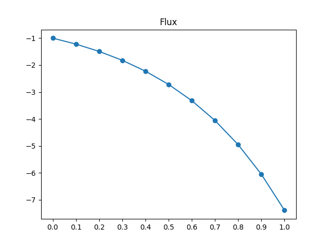
    J = np.array([-1, -math.e**(1/10)*math.e**(1/10), -math.e**(2/10)*math.e**(2/10), -math.e**(3/10)*math.e**(3/10),
                  -math.e**(4/10)*math.e**(4/10), -math.e**(5/10)*math.e**(5/10), -math.e**(6/10)*math.e**(6/10),
                  -math.e**(7/10)*math.e**(7/10), -math.e**(8/10)*math.e**(8/10), -math.e**(9/10)*math.e**(9/10),
                  -math.e**2])
    U = np.linalg.solve(A, F)
    U_hat = []
    for n in range(0, F.size):
        U_hat.append(u(n / 10))
    E = U - U_hat
    print("The solution U is:\n", U)
    print("The error of the solution is:\n", E)
    x = np.linspace(0, 1, 11)
    y = np.linspace(-0.1, 1, 12)
    plt.plot(x, U, marker='o')
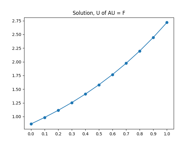
    plt.title("Solution, U of AU = F")
    plt.xticks(x)
    plt.show()
    plt.plot(x, J, marker='o')
    plt.title("Flux")
    plt.xticks(x)
    plt.show()
    plt.plot(x, E, marker='o')
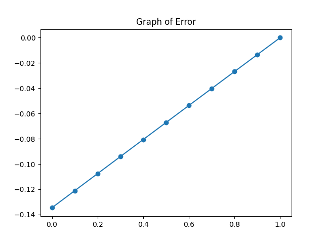
    plt.title("Graph of Error")
    plt.show()

main()

Output:

The solution U is:
 [0.86541332 0.98409843 1.11383524 1.25578609 1.41123552 1.58160319
 1.76845808 1.97353416 2.19874777 2.44621678 2.71828183]
The error of the solution is:
 [-0.13458668 -0.12107249 -0.10756752 -0.09407272 -0.08058918 -0.06711808
 -0.05366072 -0.04021854 -0.02679316 -0.01338633  0.        ]