Math5620

Author: David Merkley

Language: Python

Description/Purpose: This code solves a IVP using 2 different methods. The 4-Step Runge Kutta method and the midpoint method. It calculates the error of these solutions and plots the error. It also uses a backward Euler method to calculate a U^n+1 so the midpoint method can be used.

Implementation/Code:

from matplotlib import pyplot as plt
import numpy as np

# Function to get Exact solution
def ExactSol(t):
    return np.e ** ((1/2) * (t**2) + t)

# The initial value problem looked at
def IVP(u, t):
    return (t + 1) * u

# The backward Euler method used to calculate a U^n+1 so midpoint method can be used
def backEuler(U, t):
    return U / (1 - (0.05 * (t + 1)))

#  The midpoint method used to solve the IVP
def midpoint(U1, U2, t):
    return U1 + (0.1 * IVP(U2, t))

# All of these k functions are to evaluate the Ufinal function
def k1(U, t):
    return IVP(U, t)

def k2(U, t):
    return IVP(U + (0.05 * k1(U, t)), t + 0.05)

def k3(U, t):
    return IVP(U + (0.05 * k2(U, t)), t + 0.05)

def k4(U, t):
    return IVP(U + (0.1 * k3(U, t)), t + 0.1)

#  Returns a solution to the IVP with the Runge Kutta Method
def Ufinal(U, t):
    return U + (0.1/6 * (k1(U, t) + (2 * k2(U, t)) + (2 * k3(U, t)) + k4(U, t)))

def main():
    # Initiates lists required to plot the error of the solution
    listU = [1]
    listExact1 = [1]
    listExact2 = [1]
    listMid = [1, backEuler(1, 0.05)]
    listErrorU = []
    listErrorEuler = []

    #  For loop to get the runge kutta solution and exact solution along with it
    for n in range(1, 11):
        listU.append(Ufinal(listU[n-1], (n-1) * 0.1))
        listExact1.append(ExactSol(n * 0.1))

    # For loops to get the midpoint method solution and exact solution along with it
    for n in range(1, 20):
        listMid.append(midpoint(listMid[n-1], listMid[n], n * 0.05))
    for n in range(1, 21):
        listExact2.append(ExactSol(n * 0.05))

    # For loops to get the errors of the solutions
    for listU_i, listExact1_i in zip(listU, listExact1):
        listErrorU.append(listExact1_i - listU_i)
    for listExact2_i, listMid_i in zip(listMid, listExact2):
        listErrorEuler.append(abs(listExact2_i - listMid_i))

    # Plotting the Errors and Graphs for Comparison
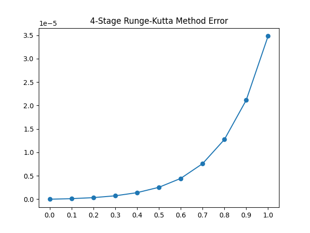
    x1 = np.linspace(0, 1, 11)
    plt.plot(x1, listErrorU, marker='o')
    plt.title("4-Stage Runge-Kutta Method Error")
    plt.xticks(x1)
    plt.show()
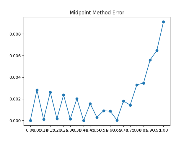
    x2 = np.linspace(0, 1, 21)
    plt.plot(x2, listErrorEuler, marker='o')
    plt.title("Midpoint Method Error")
    plt.xticks(x2)
    plt.show()
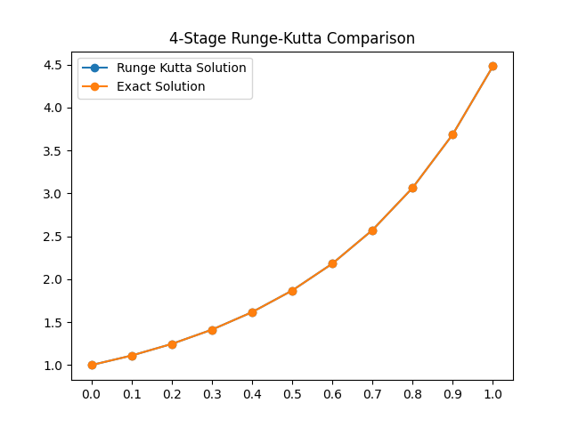
    plt.plot(x1, listU, marker='o', label='Runge Kutta Solution')
    plt.plot(x1, listExact1, marker='o', label ='Exact Solution')
    plt.legend()
    plt.title("4-Stage Runge-Kutta Comparison")
    plt.xticks(x1)
    plt.show()
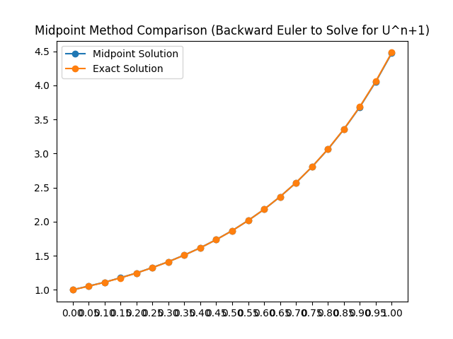
    plt.plot(x2, listMid, marker='o', label='Midpoint Solution')
    plt.plot(x2, listExact2, marker='o', label='Exact Solution')
    plt.title("Midpoint Method Comparison (Backward Euler to Solve for U^n+1)")
    plt.legend()
    plt.xticks(x2)
    plt.show()


main()

Output: